Chapter 1 - Finite element programming

I.1 Overview

The basic program structure is presented here, followed by the general idea of FEM that can be applied for all the cases and types of mechanical problems. It discusses what input data are required in general, how the global matrix equation is assembled, how the boundary conditions are applied to the matrix equation and how it is solved.

Whether we have a truss, beam, portal frame we can represent the structure as an assembly of one dimensional members, for which the exact solutions to the differential equations are known in certain special cases. In the case of a solid continuum however, such an approach does not exist in general. The solution which yields acceptable results by using discretization with the help of elements, for 2D problems: triangular or quadrilateral elements; for 3D problems: tetrahedron, or prism type of elements.

The choice sits with the analyst. However, the exact solutions to the differential equations governing the behavior of these elements are not known. To establish the relationship between the forces and displacements, the theorem of virtual work and the principle of minimum potential energy are used (weighted residual methods). Since not only the geometry, but the functional space of the solution is also discretized, in the final step, the nodal displacements are obtained through a nodal interpolation of the sought displacement field variable over the element.

The basic common principle of the finite element method in different approximation techniques is the selection of specific shape functions together by geometric and finitization.

I.2 Program structure

To understand the fundamental concepts of the finite element method, it is essential to understand the skeleton of the program structure of finite element analysis. This chapter explains the basic structure of the FEM. Finite element analysis solves an engineering problem in six (or 7 if we are as detailed as possible) steps:

1. Read input data of the already meshed geometry and allocate proper array sizes. (Geometrical finitisation).
2. Calculate element stiffness matrices and load vectors for every element. Selection of specific shape functions (Mathematical finitization).
3. Assemble element matrices and vectors into the global stiffness matrix and load vector.
4. Apply constraints to the global stiffness matrix and load vector. (Compilation of the global equation system).
5. Solve the matrix equation for the primary nodal variables (Determination of the unknown parameters, in our case displacements).
6. Compute secondary variables.
7. Plot/print desired results.

During the geometrical finitization step we divide the structure into elements (hence the name finite elements). The shape and size of the element depends a lot on the structure type itself. A plate bending problem, will need a two-dimensional division such as triangular elements or rectangular elements (more complicated shapes are not popular). If the contour is curved, we can use elements with curved sides, also we can apply different type of elements too (triangles and rectangles).

Geometrical finitzation is strongly connected to the mathematical finization, since next to the shape of the element we must decide about the number of nodes. This influences: the order of the analyzed differential equation (class of the continuity condition of the shape functions), the geometrical finitization (straight and curved elements), rate of convergence of the approximation. Next to the geometrical finitization and the selection of elements, we derive the global numbering of the nodes too.

I.3 Input data

The input parameters needed for a finite element analysis program are the following:

• the total number of nodes in the system,

• the total number of elements,

• coordinate value of nodes in terms of global coordinate system,

• type of elements,

• connectivity array,

• information for boundary conditions.

Most of these input data are associated with the finite element mesh upon which the user decides. The mesh can be generated using an automated mesh-generating program, called the pre-processor, or manually. By type of element we refer the number of nodes per element, and the degrees of freedom a node has. If the same type of element is used over the whole continua, then we only need this information for one element. It may happen that we apply different shape functions, but in most of the cases it is enough to apply one type of element and shape function family.

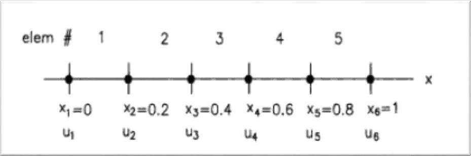
Having a simple example from reference ¹, we use one type of element to present the steps. Five equal sized linear elements are used, therefore the total number of nodes ($ nnode $) is 6 and the number of total elements in the system ($ nel $) is 5. Only x coordinates are present since it is a one-dimensional problem. $ gcoord $ denotes the array storing the coordinate values,

$ g \operatorname{coord}(1)=0.0 ; \ldots g \operatorname{coord}(2)=0.2 ; \ldots g \operatorname{coord}(3)=0.4 $

$ g \operatorname{coord}(4)=0.6 ; \ldots g \operatorname{coord}(5)=0.8 ; \ldots g \operatorname{coord}(6)=1.0 $

in which the index in the bracket is the node number which goes from 1 to 6 and the size of the vector $ gcoord $ is the same as the total number of nodes $ nnode $. The number of nodes per element is 2 ($ nnel $). The number of degrees of freedom per node ($ ndof $) is 1. The total number of degrees of freedom per system is $ sdof=nnode \times ndof $.

Information concerning the nodal connectivity for each element is an input into the program, and is called element topology. This is the basis for the evaluation of element matrices and vectors and to evaluate and assemble the system matrices. For this example, this information can be acquired in an easy way if the node numbering and element numbering are sequential from one end of the domain to the other end; 𝑛𝑜𝑑𝑒𝑠 contains the node IDs in elements, it being a two-dimensional array. The first index stands for the number of element and the second one stands for node number associated to the element. For example, in the aforementioned problem, the $i^{t h}$ element has two nodes, $i^{t h}$ and the $(i+1)^{t h}$ nodes; that is,

$nodes(i, 1)=i$ and $\operatorname{nodes}(i, 2)=i+1$ for $i=1,2,3,4,5$

The boundary of the element always has a null-size domain comparing to the element (in a 2D element the boundary line has no area). In 1D elements this is easy; we have to put the nodes at the boundaries of the elements, we prescribe a common value (1 or 0) at the same shape function.

Information regarding the boundary conditions includes the nodal degrees of freedom where constraints and external forces are applied. To specify the nodal degrees of freedom, we provide node numbers and corresponding degrees of freedom of the specified nodes.

For the present simple example these are,

$ bcdof(1)=1 $;

$ bcdof(2)=6 $.

where $bcdof$ contains the number of the constraint. The value of the constraints are given in $bcval$ in the following way,

$bcval(1)=0.0$ and $bcval(2)=0.0$.

I.4 Assembly of element matrices and vectors

In the simple example we have the element matrices and vector as functions of the length of each element. This leads to the length of each element being computed from the coordinate values of the nodes associated with the element: for ex. the $i^{t h}$ element is associated with the $i^{t h}$ and the $(i+1)^{t h}$ nodes. The coordinate values of the nodes are $gcoord(i)$ and $gcoord(i+1)$. As a result, the element length is equal to $gcoord(i+1)$ − $gcoord(i)$. If the element length is the same for the whole domain, the length can be provided as an input.

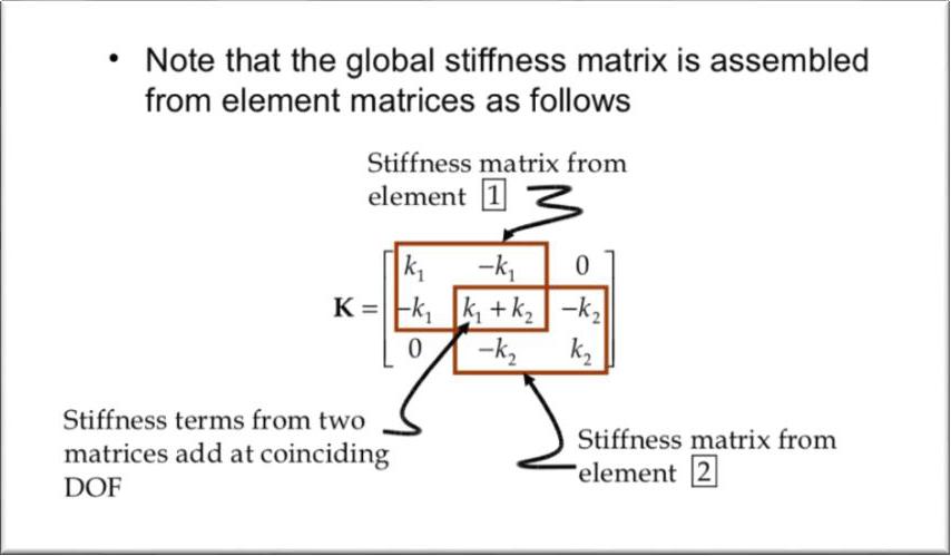
Once we compute these matrices and vectors, they need to be assembled into the system matrix and vector. Information on where the element matrix and vector are to be in the global stiffness matrix and force vector. This information is obtained from the array $index$ whose size equals to the number of degrees of freedom per element, i.e. 2 for this present example. Because each node has a single degree of freedom, the size of the array $ index $ is the same as that for array $nodes$.

Let $k$ and $f$ be the element stiffness matrix and force vector for any element. $kk$ and $ff$ are the global stiffness matrix and force vector. The array $index$ contains the degrees of freedom associated with the element. Then $k$ and $f$ are stored into $kk$ and $ff$ in the following way. This is repeated for every element.

MATLAB code:

edof=nnel*ndof; %edof=number of degrees of freedom per element
for ir=1:edof; %loop for element stiffness rows
     irs=index(ir); %address for the global stiffness row
     ff(irs)=ff(irs)+f(ir); %assembly into the force vector
     for ic=1:edof; %loop for element stiffness columns
          ics=index(ic); %address for the global stiffness column
          kk(irs,ics)=kk(irs,ics)+k(ir,ic); %assembly into the global stiffness matrix
     end %endof column loop
end %end of row loop

I.5 Application of constraints

Information on the constraints and boundary conditions is provided in arrays $bcdof$ and $bcval$ as seen in the previous subchapters. The global stiffness matrix is modified using this information. The size of the global stiffness matrix is equal to the total number of degrees of freedom in the current mechanical system. If the constraints are not applied to the system of equations the matrix equation will be singular so that it can not be inverted. In context of structural mechanics, this means that the matrix equation contains rigid body motions. If a constraint is applied to the $n^{t h}$ degree of freedom in the matrix equation, the $n^{t h}$ equation is replaced by the constraint equation. Constraining some nodes in the structure corresponds to applying boundary conditions.

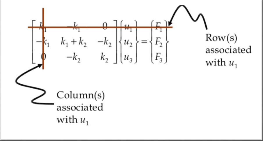
$$ \label{marker1} [k k]{u}={f f} $$

Applying the boundary conditions without destroying the symmetry:

for ic=1:2; %loop for two constaints
     id=bcdof(ic); %extract the degree of freedom for constraint
     val=bcval(ic); %extract the corresponding constrained value
     for i=1:sdof; %loop for the number of equations in the system
          ff(i)=ff(i)-val*kk(i,id) %modify column using constrainde value
          kk(id,i)=0; %set all the idth row to zero
          kk(i,id)=0; %set all of the idth column to zero
     end
     kk(id,id)=1; %set the idth diagonal to unity
     ff(id)=val; %put the constrained value in the column
end

The modified matrix equation is solved for the primary nodal unknowns. In MATLAB application this is solved as

u=kk\ff

where $ kk $ is the stiffness matrix with applied constraints.

Once the primary variable u is determined from the equation, the natural boundary conditions are found from

ff=kk*u