Chapter 4 - Framework for linear analysis of shell elements
The finite element method is frequently (if not the most) used in solving engineering problems, capable of solving various levels of shape, boundary and loading conditions with an approximate result having an acceptable level of divergence from the actual solution. When using this method, a large number of unknowns are present, which means that computer programs are needed to solve the equations. MATLAB programming language is well-suited solution for this problem. Following the steps of FEA building the framework for the linear analysis of plate/shell elements leads to more straightforward approach. The MATLAB code presented here is compiled for a quadrant of a plate element loaded transversally by a point load. This relatively simple problem was proposed to explain the structure of a FEM software by the shear simplicity that involves clarifying the programming part. This problem and its derivatives will follow the reader through the thesis, appearing in the nonlinear analysis and GUI design, which hopefully will make the task of presenting a FEM framework and comprehending the problems around it easier. Linear framework contains three parts: Preprocessor, Solver and Postprocessor, merging the steps necessary for a FEA (but omitting neither).
IV.1 Preprocessor
Preprocessor part processes the input data to produce output necessary for the Solver. It contains basic variables that are linked to the topology of the system. For our example, centered around the quadrant of a plate loaded with a point load this leads to definition of the following input data
nnel=4; % number of nodes per element
xnode=3; % number of nodes in x-axis
ynode=3; % number of nodes in y-axis
xzero=0.0; % x-coordniate of the bottom left corner
yzero=0.0; % y-coordinate of the bottom left corner
xlength=150.0; %[mm] size of domain in x-axis
ylength=150.0; %[mm] size of domain in y-axis
xnel=xnode-1; % number of elements in x-axis
ynel=ynode-1; % number of elements in y-axis
nel=xnel*ynel; % total number of elements
nnode=xnode*ynode; % total number of nodes
delx=xlength/xnel; % element size in x-axis
dely=ylength/ynel;  % element size in y-axis
The input data necessary for a linear analysis are in order of appearance: number of nodes per element (considering a
nodes=zeros(nel,nnel);
gcoord=zeros(nnode,3);
initialise matrix of nodal connectivity
Nodal coordinates are generated moving along axis x first then skipping along y and then again along x until all of the geometric constrains are reached, the size of each jump is the size of elements along x and y-axis respectively.
for iy=1:ynode
	for ix=1:xnode
	gcoord((iy-1)*xnode+ix,1)=xzero+(ix-1)*delx;
	gcoord((iy-1)*xnode+ix,2)=yzero+(iy-1)*dely;
	end
end
Nodal connectivity matrix is assembled in the following. Order of assembly is counter clockwise to prohibit the Jacobian from becoming negative (thus changing the orientation).
for iiy=1:ynel
	for iix=1:xnel
	nodes((iiy-1)*xnel+iix,1)=(iiy-1)*xnode+iix;
	nodes((iiy-1)*xnel+iix,2)=(iiy-1)*xnode+iix+1;
	nodes((iiy-1)*xnel+iix,3)=iiy*xnode+iix+1;
	nodes((iiy-1)*xnel+iix,4)=iiy*xnode+iix;
	end
end
For a mesh of 𝑔𝑐𝑜𝑜𝑟𝑑 and 𝑛𝑜𝑑𝑒𝑠 as
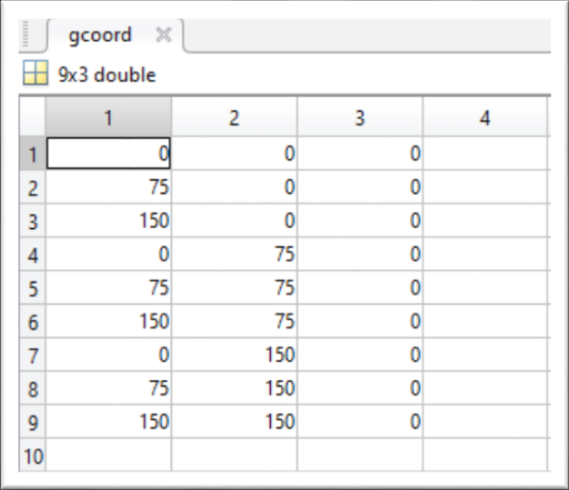
gcoord - nodal coordinates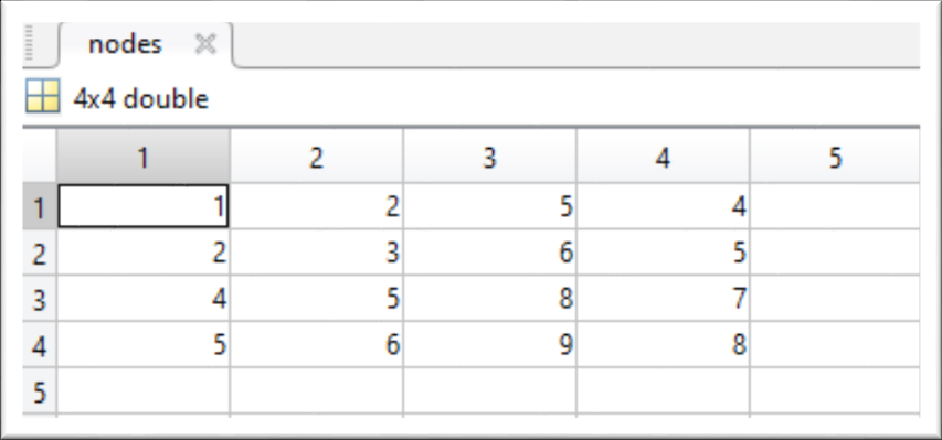
nodes - nodal connectivity matrixClosing the geometrical data input row are
ndof=6
sdof=nnode*ndof
edof=nnel*ndof
number of degrees of freedom, total number of degrees of freedom in the system and finally the number of degrees of freedom per element.
Material properties are defined: modulus of elasticity
emodule=21e4
poisson=0.3
t=5
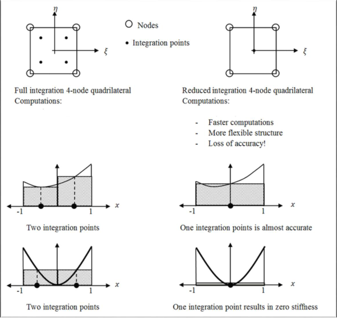
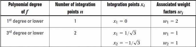
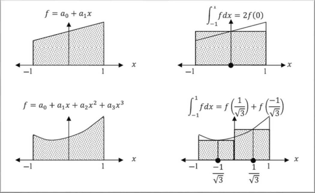
Number of Gauss-Legendre points for bending (and in-plane action) and shear are given according to the “selective” integration principle. For a 4-node quadrilateral element we have linear strains and stresses, and thus the entries in the matrix 𝐵𝑇𝐷𝐵 are quadratic functions of position. Thus, a 2×2 numerical integration scheme is required to produce accurate integrals for the isoparametric 4-node elements. This integration is called “full” integration of elements. In our example, to integrate the element stiffness matrix of size (24×24) of a quadrilateral element, each entry will be evaluated at the four locations (2×2) of the integration points of the isoparametric element. Thus, the number of computations for the integration of the element are 24×24×4=2304 computations. Because of the effect of the shear locking we will used “reduced” integration for shear calculation. The reduced integration version of a 4-node isoparametric quadrilateral element uses only one integration point in the center of the element, and the number of calculations is reduced from 2304 to 576. However, this is plagued by a loss in accuracy. In the next figure, we see two nonlinear functions integrated using one and two integration points. In the first case, the function has a small variation along the domain and the integration seems accurate. In the second case, the function has a large variation and is equal to zero in the centre of the domain. The benefit of using reduced integration is not only saving computational time, but also balancing the over-stiffness by assuming a certain deformation field within an element. However, it can lead to a structure which is too flexible.
nglxb=2 %2x2 Gauss-Legendre quadrature for
nglyb=2 %bendig-[nglxb,nglyb]
nglb=nglxb*nglyb; %number of sampling point for bending
nglxs=1 %1x1 Gauss-Legendre quadrature for
nglys=1 %shear-[nglxs,nglys]
ngls=nglxs*nglys; %number of sampling points for shear
Next steps are linked to the geometric representation of the problem topology. At the beginning
xcoord=gcoord(:,1);
ycoord=gcoord(:,2);
After which we extract the coordinates for each element to build up the borders in the graphical representation.
for i=1:nel
	for j=1:4
	x(j)=xcoord(nodes(i,j));
	y(j)=ycoord(nodes(i,j));
	end;
xvec=[x(1),x(2),x(3),x(4),x(1)];
yvec=[y(1),y(2),y(3),y(4),y(1)];
plot(xvec,yvec);
hold on;
Placing the element number on the image.
midx=mean(xvec(1:4));
midy=mean(yvec(1:4));
text(midx,midy,num2str(i));
end;
And labels for the coordinate axis.
xlabel('x axis');
ylabel('y axis');
zlabel('z axis');
title(num2str(i));
With node numbers on each node.
for jj=1:nnode
text(gcoord(jj,1),gcoord(jj,2),num2str(jj));
end;
Reaching the end of the Preprocessor by calling the patch command to represent the mesh, with element and node numbers.
patch('Faces', nodes, 'Vertices', gcoord,'Facecolor','blue',...
'FaceAlpha',.3,'Marker','.');
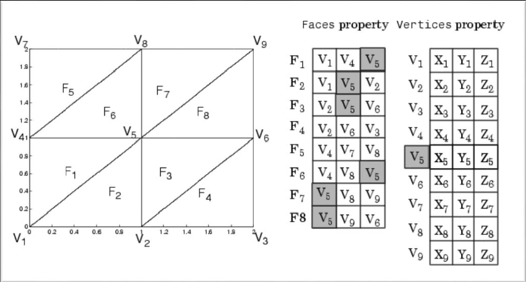
Patch (‘Faces’,F,‘Vertices’,V) creates one or more polygons where V specifies vertex values and F defines which vertices to connect. Specifying only unique vertices and their connection matrix can reduce the size of the data when there are many polygons. Specify one vertex per row in V. To create one polygon, specify F as a vector. To create multiple polygons, specify F as a matrix with one row per polygon. Each face does not have to have the same number of vertices.
Vertex connection defining each face. This property is the connection matrix specifying which vertices in the Vertices property are connected. The Faces matrix defines m faces with up to n vertices each. Each row designates the connections for a single face, and the number of elements in that row that are not NaN defines the number of vertices for that face.
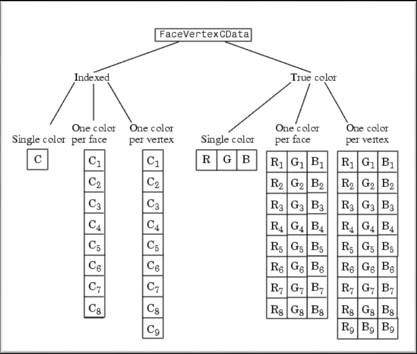
The Faces and Vertices properties provide an alternative way to specify a patch that can be more efficient than using x, y, and z coordinates in most cases. For example, consider the following patch. It is composed of eight triangular faces defined by nine vertices.
The corresponding Faces and Vertices properties are shown to the right of the patch. Note how some faces share vertices with other faces. For example, the fifth vertex (V5) is used six times, once each by faces one, two, and three and six, seven, and eight. Without sharing vertices, this same patch requires 24 vertex definitions.
Facecolor - Color of the patch face. This property can be any of the following:
ColorSpec– A three-element RGB vector or one of the MATLAB predefined names, specifying a single color for faces.none– Do not draw faces. Note that edges are drawn independently of faces.flat– TheCDataorFaceVertexCDataproperty must contain one value per face and determines the color for each face in the patch. The color data at the first vertex determines the color of the entire face.interp– Bilinear interpolation of the color at each vertex determines the coloring of each face. TheCDataorFaceVertexCDataproperty must contain one value per vertex.
patch command (Source: http://matlab.izmiran.ru/help/techdoc/ref/patch_props.html)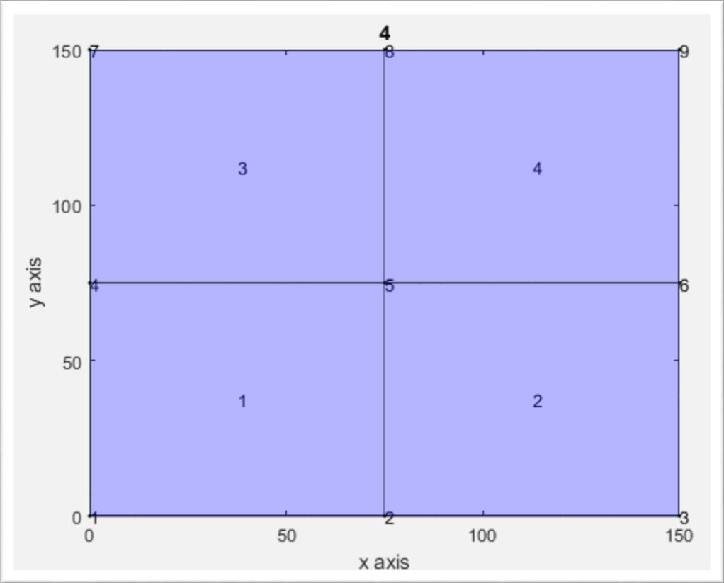
Until this point almost all the Preprocessor part was covered. The only missing elements that are necessary to be introduced are the boundary conditions and applied point loads, material property matrices for membrane, bending and shear action.
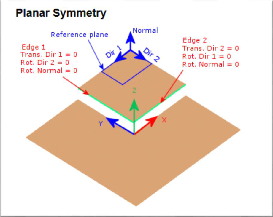
Boundary conditions for fixed along lower and left side, symmetry conditions on the upper and right side.
for i=1:nnode
if gcoord(i,1) == xzero
nf(i,1) = 0 ; % Restrain in direction u
nf(i,2) = 0 ; % Restrain in direction v
nf(i,3) = 0 ; % Restrain in driection w
nf(i,4) = 0 ; %Restrain aroundx
nf(i,5) = 0 ; %Restrain aroundy
elseif gcoord(i,2) == yzero
nf(i,1) = 0 ; % Restrain in direction u
nf(i,2) = 0 ; % Restrain in direction v
nf(i,3) = 0 ; % Restrain in driection w
nf(i,4) = 0 ; %Restrain around x
nf(i,5) = 0 ; %Restrain around y
elseif gcoord(i,1) == xlength
nf(i,1) = 0 ; %Restrain in direction u
nf(i,5) = 0 ; %Restrain around y
elseif gcoord(i,2) == ylength
nf(i,2) = 0 ; %Restrain in direction v
nf(i,4) = 0 ; %Restrain around x
end
end
Counting of the free degrees of freedom,
n=0;
for i=1:nnode
for j=1:ndof
n=n+1;
vectnf(n)=nf(i,j);
end
end
Those degrees of freedom that are constrained will be 0, the rest are 1. The size of vector vectnf is 1×54, the total number of degrees of freedom in the system.
Assembling bcdof vector,
n=0;
for i=1:sdof
	if vectnf(i)== 0
		n=n+1;
		bcdof(n)= i;
	end
end
and assigning 0 as a value for the constrained degrees of freedom,
bcval=zeros(size(bcdof))
Size of bcdof and bcval vectors is 1×31, number of the constrained degrees of freedom present.
Initialization of matrices and vectors,
ff=zeros(sdof,1); %[F] %system force vector
kk=zeros(sdof,sdof); %[K] %system matrix
delta=zeros(sdof,1); %[u] %system displacement vector
index=zeros(edof,1); %[i] %index vector
kinmtsb=zeros(3,edof); %[B_b] %kinematic matrix for bending
matmtsb=zeros(3,3); %[D_b] %constitutive matrix for bending
kinmtsm=zeros(3,edof); %[B_m] %kinematic matrix for membrane
matmtsm=zeros(3,3); %[D_m] %constitutive matrix for membrane
kinmtss=zeros(2,edof); %[B_s] %kinematic matrix for shear
matmtss=zeros(2,2); %[D_s] %constitutive matrix shear
tr3d=zeros(edof,edof); %[T] %transformation matrix
eldisp=zeros(edof,1) %[d_e] %element displacement matrix
and the force vector of -1000N along
ff(sdof-3)=-1000
Where
Using full integration for bending and membrane action, reduced integration for shear action requires the determination of the integration points and its associated weights. This is done for 1D integration and transformed into Gauss integration over two dimensional domains easily using the formula:
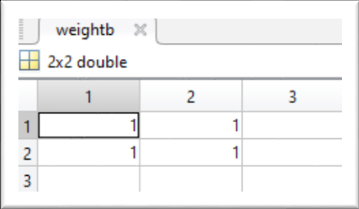
[pointb,weightb]=feglqd2(nglxb,nglyb);%sampling points & weights for bending
matmtsm=fematiso(1,emodule,poisson)*t; %membrane property [D_m]
matmtsb=fematiso(1,emodule,poisson)*t^3/12; %material property matrix [D_b]
[points,weights]=feglqd2(nglxs,nglys);%sampling points & weights for shear
shearm=0.5*emodule/(1.0+poisson); %shear modulus
shcof=5/6; %shear correction factor
matmtss=shearm*shcof*t*[1 0; 0 1]; %material property matrix
Concluding these values of matrices pointb and points are:
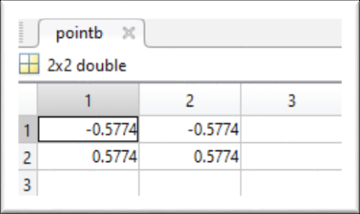
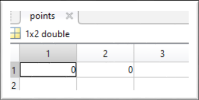
Weights are:
We also determine the material property matrices for membrane matmtsm), bending matmtsb) and shear matmtss).
These are the necessary information that can be used as an input for our solver. To sum it up as steps of FEM: Preprocessor part solved the geometrical and mathematical finitization of the problem topology. Material data was included as well as boundary conditions and vector of nodal forces, although these were not applied to our problem yet.
IV.2 Solver
The Solver for the linear analysis is built around a large loop that runs for the total number of elements. This basically covers the numerical integration for in-plane action and bending in one cycle, while shear integration is in a separate one.
for iel=1:nel
	for i=1:nnel
		nd(i)=nodes(iel,i); %extract nodes for (iel)-th element
		xcoord(i)=gcoord(nd(i),1); %extract x value of the nodes
		ycoord(i)=gcoord(nd(i),2); %extract y value of the nodes
		zcoord(i)=gcoord(nd(i),3); %extract z value of the nodes
	end
Loop start with the extraction of
While this current example does not feature 3D geometry, it has the ability to do so. We compute the local direction cosines and local axis.
[tr3d,xprime,yprime]=fetransh(xcoord,ycoord,zcoord,nnel);
tr3d Eq. (100) matrix in this case is of size 24×24 with values of 1 at its diagonal; xprime and yprime remain identical to
Initializing the matrices for stiffness in local and global axis, bending stiffness, shear stiffness and membrane stiffness:
	k=zeros(edof,edof); %element matrix in local axes
	ke=zeros(edof,edof); %element matrix in global axes
	kb=zeros(edof,edof); %bending matrix
	ks=zeros(edof,edof); %shear matrix
	km=zeros(edof,edof); %element membrane matrix
Followed by the integration loop for bending and in-plane action:
	for intx=1:nglxb
		x=pointb(intx,1); %sampling point in x-axis
		wtx=weightb(intx,1); %weight in x-axis
Two steps are to be expected according to the full integration protocol for bending. The first value for the sampling point along
Second loop inside the previous one runs along
	for inty=1:nglyb
		y=pointb(inty,2); %samplingpoint in y-axis
		wty=weightb(inty,2); %weight in y-axis

		[shape,dhdr,dhds]=feisoq4(x,y);
Shape functions feisoq4.m.
Shape functions for a four-node quadrilateral element are in the form:
Jacobian for two-dimensional mapping is assembled, fejacob.m contains the lines:
jacob2=zeros(2,2);
%
for i=1:nnel
	jacob2(1,1)=jacob2(1,1)+dhdr(i)*xcoord(i);
	jacob2(1,2)=jacob2(1,2)+dhdr(i)*ycoord(i);
	jacob2(2,1)=jacob2(2,1)+dhds(i)*xcoord(i);
	jacob2(2,2)=jacob2(2,2)+dhds(i)*ycoord(i);
end
which assembles the matrix:
The determinant and the inverse of the Jacobian:
			detjacob=det(jacob2); %determinant of Jacobian [J]
			invjacob=inv(jacob2); %inverse of Jacobian matrix
Derivatives with respect to physical coordinates by function federiv2.m:
[dhdx,dhdy]=federiv2(nnel,dhdr,dhds,invjacob);
federiv2.m containing these lines:
for i=1:nnel
	dhdx(i)=invjacob(1,1)*dhdr(i)+invjacob(1,2)*dhds(i);
	dhdy(i)=invjacob(2,1)*dhdr(i)+invjacob(2,2)*dhds(i);
end
With these data acquired we can form the kinematic matrices
			kinmtsm=fekinesm(nnel,dhdx,dhdy);%membrane kinematic mtx
			kinmtsb=fekinesb(nnel,dhdx,dhdy);%bending kinematic matrix
Thus, necessary information is available to determine element stiffness for bending action and element stiffness for in-plane action.
			kb=kb+kinmtsb'*matmtsb*kinmtsb*wtx*wty*detjacob;
			km=km+kinmtsm'*matmtsm*kinmtsm*wtx*wty*detjacob;
Numerical integration loop for the shear action is almost identical to the numerical integration of the bending part, for this we will continue to the MATLAB :TM: code, only commenting on the significant difference.
	for intx=1:nglxs
		x=points(intx,1); %sampling point in x-axis
		wtx=weights(intx,1); %weight in x-axis
		for inty=1:nglys
			y=points(inty,2); %sampling points in y-axis
			wty=weights(inty,2); %weight in y-axis
			%
			[shape,dhdr,dhds]=feisoq4(x,y);
			jacob2=fejacob2(nnel,dhdr,dhds,xprime,yprime);%Jacobian
			detjacob=det(jacob2);
			invjacob=inv(jacob2);
			[dhdx,dhdy]=federiv2(nnel,dhdr,dhds,invjacob);
Shear kinematic matrix is assembled in place of the bending and membrane terms:
kinmtss=fekiness(nnel,dhdx,dhdy,shape);%shear kinematicmtx
Element shear stiffness can be written in the form:
ks=ks+kinmtss'*matmtss*kinmtss*wtx*wty*detjacob;
Loop for the integration ends here, successively continuing the loop on the lower order of priority to the next element.
When this loop terminates also, (element stiffness of all the elements was determined) we can compute the total element stiffness matrix
k=km+kb+ks;
We do the transformation from local to global systems (in this example, it is irrelevant):
ke=tr3d’*k*tr3d;
Associated degrees of freedom are extracted:
index=feeldof(nd,nnel,ndof);
feeldof.m function contains the following code:
k=0;
for i=1:nnel
start=(nd(i)-1)*ndof;
	for j=1:ndof
		k=k+1;
		index(k)=start+j;
	end
end
It gets the number of the degree of freedom associated to each node (For ex. node 3 has the degrees of freedom 13,14,15,16,17,18) The next step is to assemble global stiffness matrix:
kk=feasmbl1(kk,ke,index);
feasmbl1.m function contains the lines:
edof=length(index);
for i=1:edof
	ii=index(i);
	for j=1:edof
		jj=index(j);
		kk(ii,jj)=kk(ii,jj)+k(i,j);
	end
end
Boundary conditions are applied to the stiffness matrix.
[kk,ff]=feaplyc2(kk,ff,bcdof,bcval);
Running for the number of constrains, for each degree of freedom constrained, we change tha values of entries kk(nr. of dof, nr. of dof of the system)=0 and kk(nr. of dof, nr. of dof)=0, with values in the force vector ff(nr. of dof)=0 also. feaplyc2.m function contains the lines:
n=length(bcdof);
sdof=size(kk);
%
for i=1:n
	c=bcdof(i);
	for j=1:sdof
		kk(c,j)=0;
	end
	%
	kk(c,c)=1;
	ff(c)=bcval(i);
end
Finally we arrive at the end of the Solver. This contains the system of linear equation in the form:
We solve the system of linear equation for
delta=kk\ff;
The vector of the displacement for current example is of the size 54×1.
IV.3 Postprocessor
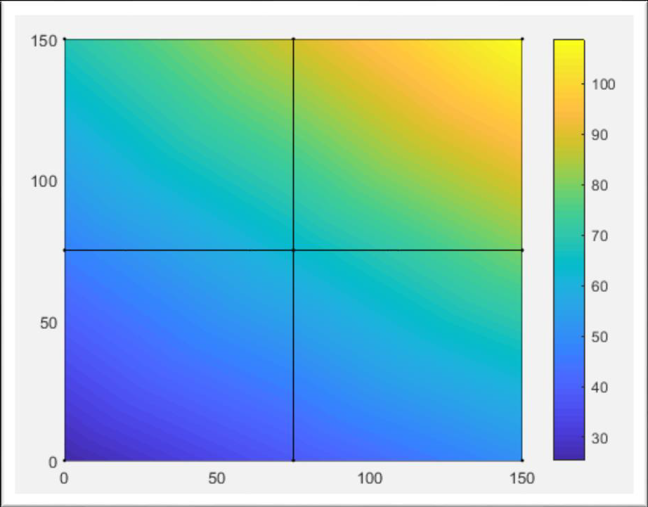
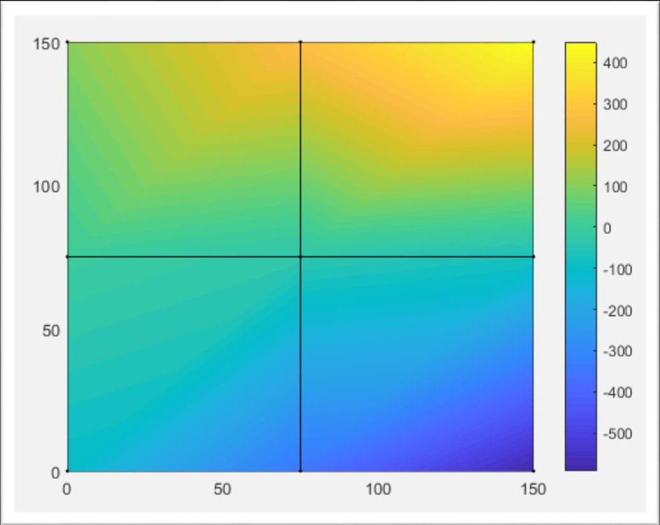
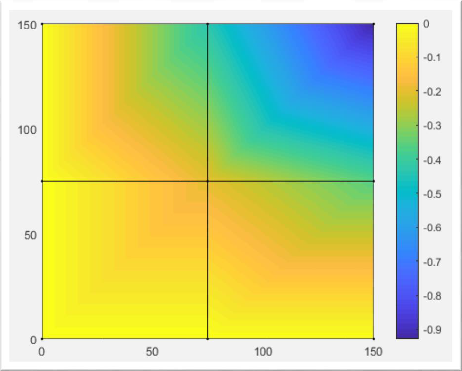
Postprocessor part is the one which uses the output of the Solver to process the data in a human readable form. This includes figures and the calculation of the secondary variables. For the current example, the start of the Postprocessor is marked by the command patch, illustrating the displacement along axis
patch('Faces', nodes, 'Vertices', gcoord,'FaceVertexCData',...
	delta(3:6:end),'FaceColor','interp','FaceAlpha',1,'Marker','.');
colorbar
c1=min(delta(3:6:end))
Every third value (dof 'FaceVertexCData':
Face and vertex colors. The FaceVertexCData property specifies the color of patches defined by the Faces and Vertices properties. You must also set the values of the FaceColor, EdgeColor, MarkerFaceColor, or MarkerEdgeColor are set appropriately. The interpretation of the values specified for FaceVertexCData depends on the dimensions of the data.
For indexed colors, FaceVertexCData can be
- A single value, which applies a single color to the entire patch
- An n-by-1 matrix, where n is the number of rows in the
Facesproperty, which specifies one color per face - An n-by-1 matrix, where n is the number of rows in the
Verticesproperty, which specifies one color per vertex
For true colors, FaceVertexCData can be
- A 1-by-3 matrix, which applies a single color to the entire patch
- An n-by-3 matrix, where n is the number of rows in the
Facesproperty, which specifies one color per face - An n-by-3 matrix, where n is the number of rows in the
Verticesproperty, which specifies one color per vertex
The following diagram illustrates the various forms of the FaceVertexCData property for a patch having eight faces and nine vertices. The CDataMapping property determines how MATLAB interprets the FaceVertexCData property when you specify indexed colors.
Displacements are:
The next major step, that will be familiar for the reader is the calculation of the element stresses. The same integration scheme (that appears at the bending and shear) will be used for this purpose also. Individual steps that are reused from previous code lines will not be further discussed.
for ielp=1:nel %loop for the total number of elements
	for i=1:nnel
		nd(i)=nodes(ielp,i); %extract for (iel)-th element
		xcoord(i)=gcoord(nd(i),1); %extract x value of the node
		ycoord(i)=gcoord(nd(i),2); %extract y value of the node
	end

ngl=1; %integration in the middle of the element
for intx=1:ngl
		x=points(intx,1); %sampling point in x-axis
		wtx=weights(intx,1); %weight in x-axis
		for inty=1:ngl
			y=points(inty,2); %samplingpoint in y-axis
			wty=weights(inty,2); %weight in y-axis
			%
			[shape,dhdr,dhds]=feisoq4(x,y); %compute shape functions and derivatives at sampling point
			%
			jacob2=fejacob2(nnel,dhdr,dhds,xprime,yprime);
			% %Jacobian matrix
			detjacob=det(jacob2); %determinant of Jacobian
			invjacob=inv(jacob2); %inverse of Jacobian
			%
			[dhdx,dhdy]=federiv2(nnel,dhdr,dhds,invjacob); %derivatives w.r.t psysical coordinates
All the kinematic matrices are initialized 𝐵_{𝑚},𝐵_{𝑏},𝐵_{𝑠}:
			kinmtsm=fekinesm(nnel,dhdx,dhdy);%membrane kinematic mtx
			kinmtsb=fekinesb(nnel,dhdx,dhdy);%bending kinematic mtx
			kinmtss=fekiness(nnel,dhdx,dhdy,shape);%shear kinematic mx
Extracting the degrees of freedom associated with each element:
index=feeldof(nd,nnel,ndof);
Displacements associated with the element degrees of freedom:
			for iedof=1:edof
			eldisp(iedof)=delta(index(iedof));
			end
Normal curvatures are determined:
chi_m=kinmtsm*eldisp;
From this result the normal forces:
Normal=matmtsm*chi_m;
Bending curvatures have the form:
chi_b=kinmtsb*eldisp;
From here we have the bending moments:
Moment=matmtsb*chi_b;
Shear curvatures:
chi_s=kinmtss*eldisp;
Shear forces:
Shear=matmtss*chi_s;
Before proceeding on to the next element, the value of the element forces is recorded:
Element_forces(ielp,:)=[Normal' Moment' Shear'];
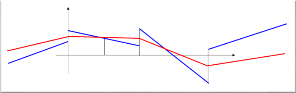
After the loop finishes, we calculate the forces at nodes. Since strains are obtained by taking first order derivatives of displacements, strains and stresses have a lower accuracy than displacements.
Since the integrals in finite element are carried out on Gauss integral points, the stresses and strains have higher accuracy when calculated on Gauss points than when calculated on nodal points.
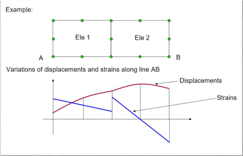
Displacements are continuous across the elements, while the strains are non-continuous.
Strains calculated based on element displacement fields will not be smooth. This is represented in the following figure.
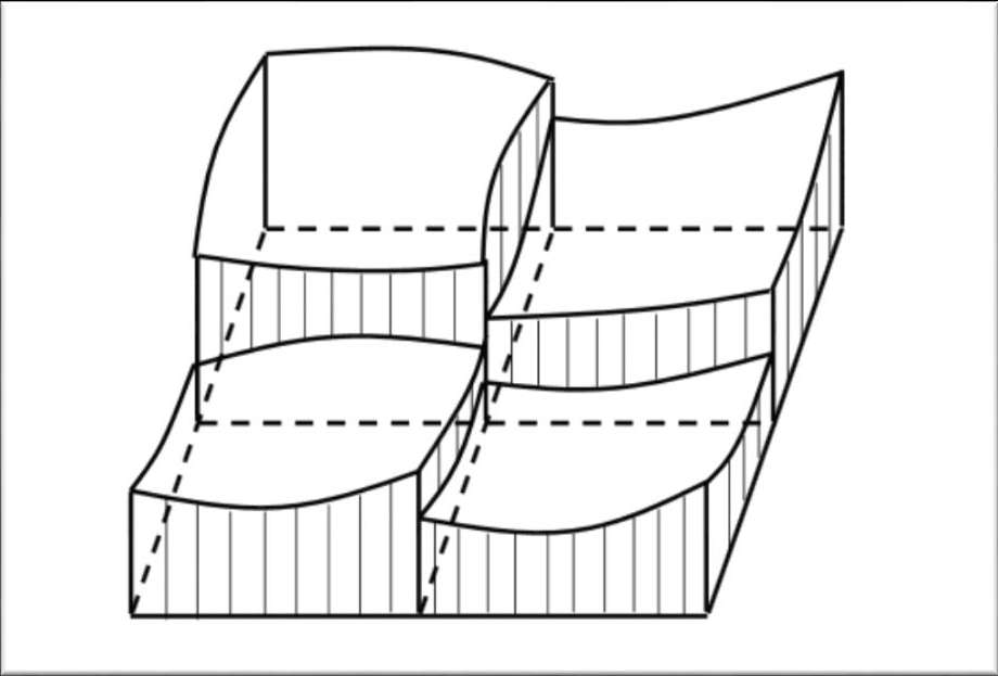
Smoothing of the strain fields and stress fields is achieved by simply averaging the nodal strains and stresses.
For this purpose, we call in the function Forces_at_nodes_shell.m:
[NX, NY, NXY, MX, MY, MXY, QX, QY]=Forces_at_nodes_shell(Element_forces,nnode,nel,nnel,nodes);
Containing the code to average the element forces while returning the values for each force:
for k = 1:nnode
	nx = 0. ; ny = 0. ; nxy = 0. ;
	mx = 0. ; my = 0. ; mxy = 0. ;
	qx = 0. ; qy = 0. ;
	ne = 0;
	for ielforce = 1:nel;
		for jelforce=1:nnel;
			if nodes(ielforce,jelforce) == k;
				ne=ne+1;
				nx = nx + Element_Forces(ielforce,1);
				ny = ny + Element_Forces(ielforce,2);
				nxy= nxy + Element_Forces(ielforce,3);
				mx = mx + Element_Forces(ielforce,4);
				my = my + Element_Forces(ielforce,5);
				mxy = mxy + Element_Forces(ielforce,6);
				qx = qx + Element_Forces(ielforce,7);
				qy = qy + Element_Forces(ielforce,8);
			end
		end
	end
	NX(k,1) = nx/ne;
	NY(k,1) = ny/ne;
	NXY(k,1)= nxy/ne;
	MX(k,1) = mx/ne;
	MY(k,1) = my/ne;
	MXY(k,1) = mxy/ne;
	QX(k,1) = qx/ne;
	QY(k,1) = qy/ne;
end
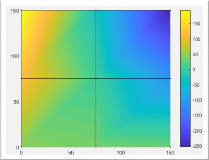
This concludes our linear solver. The last steps for the Postprocessor are the instances to display the figures for each force:
figure('Name','NX-normal force [N]');
cmin1 = min(NX);
cmax1 = max(NX);
caxis([cmin1 cmax1]);
patch('Faces', nodes, 'Vertices', gcoord, 'FaceVertexCData',NX,'Facecolor','interp','Marker','.');
colorbar;
nxmin=cmin1
nxmax=cmax1
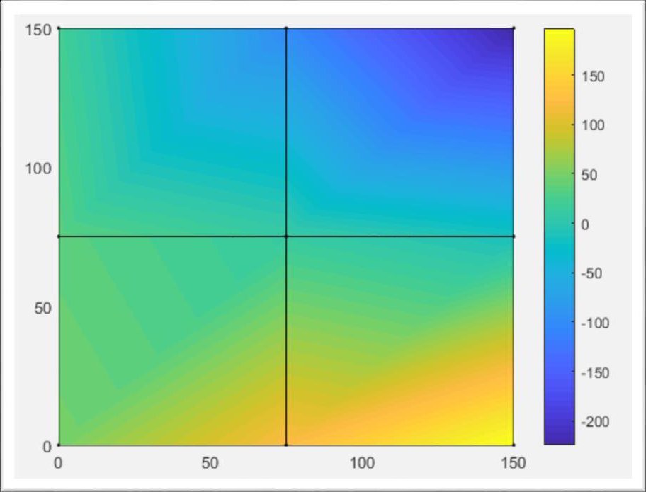
figure('Name','NY-normal force [N]');
cmin2 = min(NY);
cmax2 = max(NY);
caxis([cmin2 cmax2]);
patch('Faces', nodes, 'Vertices', gcoord, 'FaceVertexCData',NY,'Facecolor','interp','Marker','.');
colorbar;
nymin=cmin2
nymax=cmax2
figure('Name','NXY-normal force [N]');
cmin3 = min(NXY);
cmax3 = max(NXY);
caxis([cmin3 cmax3]);
patch('Faces', nodes, 'Vertices', gcoord, 'FaceVertexCData',NXY,'Facecolor','interp','Marker','.');
colorbar;
nxymin=cmin3
nxymax=cmax3
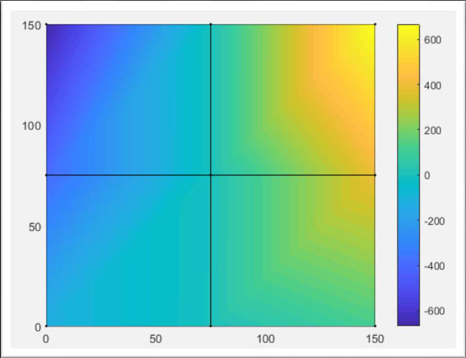
figure('Name','MX-bending moment [Nmm]');
cmin4 = min(MX);
cmax4 = max(MX);
caxis([cmin4 cmax4]);
patch('Faces', nodes, 'Vertices', gcoord, 'FaceVertexCData',MX,'Facecolor','interp','Marker','.');
colorbar;
mxmin=cmin4
mxmax=cmax4
Name','MY-bending moment [Nmm]');
cmin5 = min(MY);
cmax5 = max(MY);
caxis([cmin5 cmax5]);
patch('Faces', nodes, 'Vertices', gcoord, 'FaceVertexCData',MY,'Facecolor','interp','Marker','.');
colorbar;
mymin=cmin5
mymax=cmax5
figure('Name','MXY-bending moment [Nmm]');
cmin6 = min(MXY);
cmax6 = max(MXY);
caxis([cmin6 cmax6]);
patch('Faces', nodes, 'Vertices', gcoord, 'FaceVertexCData',MXY,'Facecolor','interp','Marker','.');
colorbar;
mxymin=cmin6
mxymax=cmax6
figure('Name','QX-shear force [N]');
cmin7 = min(QX);
cmax7 = max(QX);
caxis([cmin7 cmax7]);
patch('Faces', nodes, 'Vertices', gcoord, 'FaceVertexCData',QX,'Facecolor','interp','Marker','.');
colorbar;
qxmin=cmin7
qxmax=cmax7
figure('Name','QY-shear force [N]');
cmin8 = min(QY);
cmax8 = max(QY);
caxis([cmin8 cmax8]);
patch('Faces', nodes, 'Vertices', gcoord, 'FaceVertexCData',QY,'Facecolor','interp','Marker','.');
colorbar;
qymin=cmin8
qymax=cmax8